Difference between revisions of "RDF Graph Model"
(→RDF Datasets) |
(→BI) |
||
| (14 intermediate revisions by the same user not shown) | |||
| Line 1: | Line 1: | ||
= RDF Graph Model = | = RDF Graph Model = | ||
| − | We propose a new formal model for representing any set of RDF triples as | + | We propose a new formal model for representing any set of RDF triples as a labeled directed multigraph, or LDM. Two existing approaches use either Node-LabeledArc-Node (NLAN) diagram or Bipartite (BI) graph. |
| + | We demonstrate the three approaches using the following example. | ||
== Example == | == Example == | ||
| Line 53: | Line 54: | ||
== More complex examples == | == More complex examples == | ||
| − | [[Singleton_Property]] approach to | + | We use [[Singleton_Property]] approach to represent the duration of the marriage between Bob Dylan and Sara Lownds. |
[[File:Example_ldm_sp.png|400px|This figure demonstrates the new approach for representing a more complex fact as a labeled directed multigraph]] | [[File:Example_ldm_sp.png|400px|This figure demonstrates the new approach for representing a more complex fact as a labeled directed multigraph]] | ||
| Line 64: | Line 65: | ||
* BKR-SP: created by Vinh Nguyen et al. [http://dl.acm.org/citation.cfm?id=2567973 ACM]. This dataset is available at [[Singleton_Property]]. | * BKR-SP: created by Vinh Nguyen et al. [http://dl.acm.org/citation.cfm?id=2567973 ACM]. This dataset is available at [[Singleton_Property]]. | ||
* YAGO2S-SP: also created by Vinh Nguyen et al. [http://dl.acm.org/citation.cfm?id=2567973 ACM]. This dataset is also available at [[Singleton_Property]] | * YAGO2S-SP: also created by Vinh Nguyen et al. [http://dl.acm.org/citation.cfm?id=2567973 ACM]. This dataset is also available at [[Singleton_Property]] | ||
| − | * DBPedia 3.9: download at [http://wiki.dbpedia.org/Downloads39] | + | * DBPedia 3.9: download at [http://wiki.dbpedia.org/Downloads39 DBPedia39] |
| − | * Freebase: download at [https://developers.google.com/freebase/data]. For our experiment, we downloaded this dataset on March 30. | + | * Freebase: download at [https://developers.google.com/freebase/data Freebase]. For our experiment, we downloaded this dataset on March 30. |
| − | == Experimental | + | == Experimental Result Files == |
| − | == Degree distributions == | + | We created multiple MapReduce jobs to compute the degree distributions of all three approaches on four RDF datasets. |
| + | |||
| + | * [https://drive.google.com/file/d/0B5AIWZ9-TifAelNpTlJmeEFNT2c/edit?usp=sharing LDM degree distribution files] | ||
| + | * [https://drive.google.com/file/d/0B5AIWZ9-TifAVEY4R0hSY3dUN0E/edit?usp=sharing BI degree distribution files] | ||
| + | * [https://drive.google.com/file/d/0B5AIWZ9-TifAeG8xWWlidmNJZGs/edit?usp=sharing NLAN degree distribution files] | ||
| + | |||
| + | == Plotting Degree distributions == | ||
| + | |||
| + | Here we plot the degree distributions of three approaches (LDM, NLAN, BI) on four RDF datasets. | ||
| + | |||
| + | For each dataset, we compute in-degree, out-degree, and total-degree distributions for LDM and NLAN approaches. BI approach has only total-degree distribution because it is undirected graph. We also compare the power law fit vs. exponential fit for each plot. | ||
=== LDM === | === LDM === | ||
| + | |||
| + | {| class="wikitable" | ||
| + | ! DS | ||
| + | ! Degree type | ||
| + | ! alpha | ||
| + | ! xmin | ||
| + | ! sigma | ||
| + | ! R | ||
| + | ! p | ||
| + | ! D min | ||
| + | ! Tail coverage | ||
| + | |- | ||
| + | | rowspan="3" | BKR | ||
| + | | in | ||
| + | | 1.12 | ||
| + | | 1 | ||
| + | | 0.02 | ||
| + | | 6.78 | ||
| + | | 1.24E-11 | ||
| + | | 0.15 | ||
| + | | 60% | ||
| + | |- | ||
| + | | out | ||
| + | | 1.23 | ||
| + | | 1024 | ||
| + | | 0.04 | ||
| + | | 4.01 | ||
| + | | 6.10E-05 | ||
| + | | 0.14 | ||
| + | | 28% | ||
| + | |- | ||
| + | | total | ||
| + | | 1.21 | ||
| + | | 955 | ||
| + | | 0.04 | ||
| + | | 3.95 | ||
| + | | 7.87E-05 | ||
| + | | 0.13 | ||
| + | | 58.33% | ||
| + | |- | ||
| + | | rowspan="3" | YAGO2S | ||
| + | | in | ||
| + | | 1.11 | ||
| + | | 1 | ||
| + | | 0.02 | ||
| + | | 6.33 | ||
| + | | 2.52E-10 | ||
| + | | 0.14 | ||
| + | | 96.3% | ||
| + | |- | ||
| + | | out | ||
| + | | 1.11 | ||
| + | | 1 | ||
| + | | 0.02 | ||
| + | | 5.98 | ||
| + | | 2.18E-09 | ||
| + | | 0.14 | ||
| + | | 96.3% | ||
| + | |- | ||
| + | | total | ||
| + | | 1.13 | ||
| + | | 4 | ||
| + | | 0.02 | ||
| + | | 6.36 | ||
| + | | 2.03E-10 | ||
| + | | 0.12 | ||
| + | | 92.31% | ||
| + | |- | ||
| + | | rowspan="3" | DBPEDIA | ||
| + | | in | ||
| + | | 1.49 | ||
| + | | 974383 | ||
| + | | 0.13 | ||
| + | | 1.76 | ||
| + | | 0.08 | ||
| + | | 0.11 | ||
| + | | 25% | ||
| + | |- | ||
| + | | out | ||
| + | | 1.46 | ||
| + | | 524288 | ||
| + | | 0.11 | ||
| + | | 2.47 | ||
| + | | 0.01 | ||
| + | | 0.12 | ||
| + | | 28.57% | ||
| + | |- | ||
| + | | total | ||
| + | | 1.13 | ||
| + | | 16 | ||
| + | | 0.02 | ||
| + | | 5.38 | ||
| + | | 7.39E-08 | ||
| + | | 0.15 | ||
| + | | 85.19% | ||
| + | |- | ||
| + | | rowspan="3" | FREEBASE | ||
| + | | in | ||
| + | | 1.16 | ||
| + | | 256 | ||
| + | | 0.02 | ||
| + | | 5.56 | ||
| + | | 2.65E-08 | ||
| + | | 0.11 | ||
| + | | 70% | ||
| + | |- | ||
| + | | out | ||
| + | | 1.81 | ||
| + | | 16777216 | ||
| + | | 0.26 | ||
| + | | 1.54 | ||
| + | | 0.12 | ||
| + | | 0.12 | ||
| + | | 16.67% | ||
| + | |- | ||
| + | | total | ||
| + | | 1.14 | ||
| + | | 64 | ||
| + | | 0.02 | ||
| + | | 5.91 | ||
| + | | 3.51E-09 | ||
| + | | 0.12 | ||
| + | | 79.31% | ||
| + | |} | ||
==== BKR-SP ==== | ==== BKR-SP ==== | ||
| Line 106: | Line 241: | ||
=== NLAN === | === NLAN === | ||
| + | This table shows the parameters of the best power law distributions for each datasets using the NLAN approach. | ||
{| class="wikitable" | {| class="wikitable" | ||
| Line 116: | Line 252: | ||
! R | ! R | ||
! p | ! p | ||
| + | ! Tail Coverage | ||
|- | |- | ||
| rowspan="3" style="text-align: center;" | BKR-SP | | rowspan="3" style="text-align: center;" | BKR-SP | ||
| Line 125: | Line 262: | ||
| 2.271051161 | | 2.271051161 | ||
| 0.023143881 | | 0.023143881 | ||
| + | | 12.5% | ||
|- | |- | ||
| out | | out | ||
| Line 133: | Line 271: | ||
| 3.894424558 | | 3.894424558 | ||
| 9.84E-05 | | 9.84E-05 | ||
| + | | 31.58% | ||
|- | |- | ||
| total | | total | ||
| Line 141: | Line 280: | ||
| 3.228857504 | | 3.228857504 | ||
| 0.001242858 | | 0.001242858 | ||
| + | | 58.33% | ||
|- | |- | ||
| rowspan="3" | YAGO2S-SP | | rowspan="3" | YAGO2S-SP | ||
| Line 150: | Line 290: | ||
| 6.236336995 | | 6.236336995 | ||
| 4.48E-10 | | 4.48E-10 | ||
| + | | 92.31% | ||
|- | |- | ||
| out | | out | ||
| Line 158: | Line 299: | ||
| 4.997441147 | | 4.997441147 | ||
| 5.81E-07 | | 5.81E-07 | ||
| + | | 73.33% | ||
|- | |- | ||
| total | | total | ||
| Line 166: | Line 308: | ||
| 5.732859944 | | 5.732859944 | ||
| 9.88E-09 | | 9.88E-09 | ||
| + | | 84.62% | ||
|- | |- | ||
| rowspan="3" | DBPEDIA | | rowspan="3" | DBPEDIA | ||
| Line 175: | Line 318: | ||
| 1.899457176 | | 1.899457176 | ||
| 0.057504392 | | 0.057504392 | ||
| + | | 12.5% | ||
|- | |- | ||
| out | | out | ||
| Line 183: | Line 327: | ||
| 2.574136552 | | 2.574136552 | ||
| 0.01004906 | | 0.01004906 | ||
| + | | 0% | ||
|- | |- | ||
| total | | total | ||
| Line 191: | Line 336: | ||
| 1.774194648 | | 1.774194648 | ||
| 0.076030959 | | 0.076030959 | ||
| + | | 12.5% | ||
|- | |- | ||
| rowspan="3" | FREEBASE | | rowspan="3" | FREEBASE | ||
| Line 200: | Line 346: | ||
| 4.937155187 | | 4.937155187 | ||
| 7.93E-07 | | 7.93E-07 | ||
| + | | 64.29% | ||
|- | |- | ||
| out | | out | ||
| Line 208: | Line 355: | ||
| 6.185548611 | | 6.185548611 | ||
| 6.19E-10 | | 6.19E-10 | ||
| + | | 96.3% | ||
|- | |- | ||
| total | | total | ||
| Line 216: | Line 364: | ||
| 5.311427686 | | 5.311427686 | ||
| 1.09E-07 | | 1.09E-07 | ||
| + | | 77.78% | ||
|} | |} | ||
| Line 225: | Line 374: | ||
File:Nlan_bkr_out.png|Out-degree distribution. | File:Nlan_bkr_out.png|Out-degree distribution. | ||
File:Nlan_bkr_total.png|Total-degree distribution. | File:Nlan_bkr_total.png|Total-degree distribution. | ||
| + | </gallery> | ||
| + | |||
| + | ==== YAGO2S-SP ==== | ||
| + | |||
| + | <gallery perrow=3 widths=320px heights=240px caption="NLAN graphs transformed from the YAGO2S-SP dataset"> | ||
| + | File:Nlan_yago_in.png|In-degree distribution. | ||
| + | File:Nlan_yago_out.png|Out-degree distribution. | ||
| + | File:Nlan_yago_total.png|Total-degree distribution. | ||
</gallery> | </gallery> | ||
| Line 241: | Line 398: | ||
File:Nlan_freebase_out.png|Out-degree distribution. | File:Nlan_freebase_out.png|Out-degree distribution. | ||
File:Nlan_freebase_total.png|Total-degree distribution. | File:Nlan_freebase_total.png|Total-degree distribution. | ||
| − | |||
| − | |||
| − | |||
| − | |||
| − | |||
| − | |||
| − | |||
| − | |||
</gallery> | </gallery> | ||
=== BI === | === BI === | ||
| + | This table shows the parameters of the best power law distributions for each datasets using the BI approach. | ||
{| class="wikitable" | {| class="wikitable" | ||
| Line 261: | Line 411: | ||
! R | ! R | ||
! p | ! p | ||
| + | ! Tail Coverage | ||
|- | |- | ||
| BKR | | BKR | ||
| Line 269: | Line 420: | ||
| 4.762452101 | | 4.762452101 | ||
| 1.91E-06 | | 1.91E-06 | ||
| + | | 62.5% | ||
|- | |- | ||
| Yago2s | | Yago2s | ||
| Line 277: | Line 429: | ||
| 6.136824765 | | 6.136824765 | ||
| 8.42E-10 | | 8.42E-10 | ||
| + | | 92.31% | ||
|- | |- | ||
| DBpedia | | DBpedia | ||
| Line 285: | Line 438: | ||
| 2.766134059 | | 2.766134059 | ||
| 0.005672521 | | 0.005672521 | ||
| + | | 26.93% | ||
|- | |- | ||
| Freebase | | Freebase | ||
| Line 293: | Line 447: | ||
| 2.006340037 | | 2.006340037 | ||
| 0.044819981 | | 0.044819981 | ||
| + | | 13.79% | ||
|} | |} | ||
| Line 303: | Line 458: | ||
File:Bi_freebase_total.png|FREEBASE total-degree distribution | File:Bi_freebase_total.png|FREEBASE total-degree distribution | ||
</gallery> | </gallery> | ||
| + | |||
| + | == Comparison == | ||
| + | |||
| + | This table compares the power-law degree distribution of three type of graphs (NLAN, LDM, and BI) based on four RDF datasets (BKR, YAGO2S, DBPEDIA and FREEBASE. | ||
| + | The values are the percentage of data points in each degree distribution that are covered by the power law. Distribution with higher percentage will better reflect power law distribution in the tail. | ||
| + | |||
| + | {| class="wikitable" | ||
| + | ! DS | ||
| + | ! degree | ||
| + | ! NLAN | ||
| + | ! LDM | ||
| + | ! BI | ||
| + | |- | ||
| + | | rowspan="3" | BKR | ||
| + | | in | ||
| + | | 12.5% | ||
| + | | 60% | ||
| + | | NA | ||
| + | |- | ||
| + | | out | ||
| + | | 31.58% | ||
| + | | 28% | ||
| + | | NA | ||
| + | |- | ||
| + | | total | ||
| + | | 58.33% | ||
| + | | 58.33% | ||
| + | | 62.5% | ||
| + | |- | ||
| + | | rowspan="3" | YAGO2S | ||
| + | | in | ||
| + | | 92.31% | ||
| + | | 96.3% | ||
| + | | NA | ||
| + | |- | ||
| + | | out | ||
| + | | 73.33% | ||
| + | | 96.3% | ||
| + | | NA | ||
| + | |- | ||
| + | | total | ||
| + | | 84.62% | ||
| + | | 92.31% | ||
| + | | 92.31% | ||
| + | |- | ||
| + | | rowspan="3" | DBPEDIA | ||
| + | | in | ||
| + | | 12.5% | ||
| + | | 25% | ||
| + | | NA | ||
| + | |- | ||
| + | | out | ||
| + | | 0% | ||
| + | | 28.57% | ||
| + | | NA | ||
| + | |- | ||
| + | | total | ||
| + | | 12.5% | ||
| + | | 85.19% | ||
| + | | 29.63% | ||
| + | |- | ||
| + | | rowspan="3" | FREEBASE | ||
| + | | in | ||
| + | | 64.29% | ||
| + | | 70% | ||
| + | | NA | ||
| + | |- | ||
| + | | out | ||
| + | | 96.3% | ||
| + | | 16.67% | ||
| + | | NA | ||
| + | |- | ||
| + | | total | ||
| + | | 77.78% | ||
| + | | 79.31% | ||
| + | | 13.79 | ||
| + | |} | ||
| + | |||
| + | === LDM and NLAN === | ||
| + | |||
| + | In general, LDM distributions have higher coverage percentage than the NLAN graphs. Out of 12 degree distributions, 9 LDM distributions have higher coverage than NLAN distributions while only 2 NLAN distributions have higher percentage. Both share the same coverage for BKR total degree distribution. | ||
| + | Especially for all the in-degree and total-degree distributions, 100% LDM distributions have higher percentage than the NLAN distributions. | ||
| + | |||
| + | === LDM and BI === | ||
| + | |||
| + | 2 out of 4 LDM graphs have significantly higher coverage percentage than the BI graphs, particularly in the total degree distributions of DBPedia (LDM: 85.19% vs. BI: 29.63%) and Freebase (LDM: 79.31% vs. BI: 13.79%). | ||
Latest revision as of 08:40, 12 June 2014
Contents
RDF Graph Model
We propose a new formal model for representing any set of RDF triples as a labeled directed multigraph, or LDM. Two existing approaches use either Node-LabeledArc-Node (NLAN) diagram or Bipartite (BI) graph. We demonstrate the three approaches using the following example.
Example
| Triple | Subject | Predicate | Object |
|---|---|---|---|
| T1 | BobDylan | isMarriedTo | SaraLownds |
| T2 | BarackObama | isMarriedTo | MichelleObama |
| T3 | isMarriedTo | rdfs:subPropertyOf | isSpouseOf |
| T4 | BobDylan | isSpouseOf | SaraLownds |
| T5 | BarackObama | isSpouseOf | MichelleObama |
For the set of RDF triples in the table above, we explain how each approach represents them in the graph.
The NLAN model

The BI model

The LDM model

More complex examples
We use Singleton_Property approach to represent the duration of the marriage between Bob Dylan and Sara Lownds.

Empirical studies
RDF Datasets
We use four RDF datasets that are publicly available on the Web.
- BKR-SP: created by Vinh Nguyen et al. ACM. This dataset is available at Singleton_Property.
- YAGO2S-SP: also created by Vinh Nguyen et al. ACM. This dataset is also available at Singleton_Property
- DBPedia 3.9: download at DBPedia39
- Freebase: download at Freebase. For our experiment, we downloaded this dataset on March 30.
Experimental Result Files
We created multiple MapReduce jobs to compute the degree distributions of all three approaches on four RDF datasets.
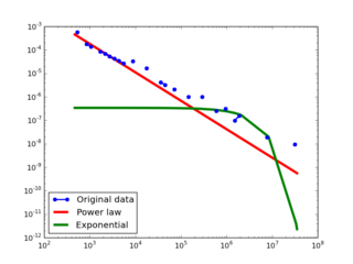
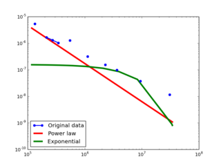
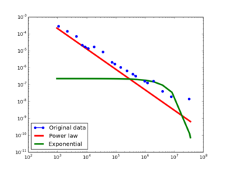
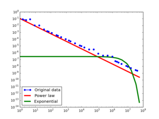
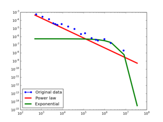
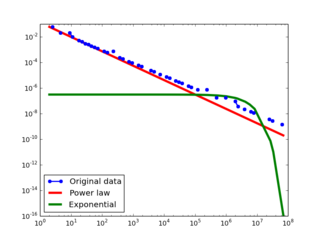
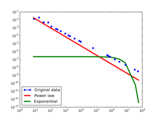
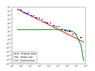
Plotting Degree distributions
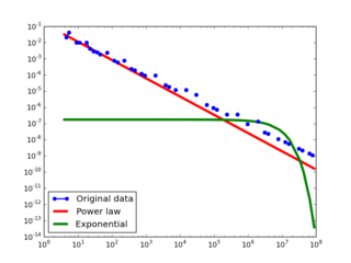
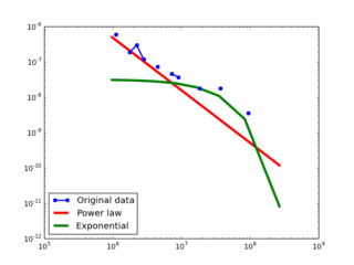
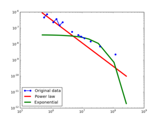
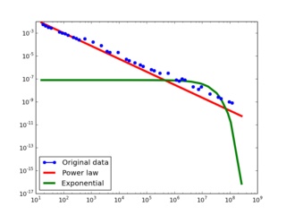
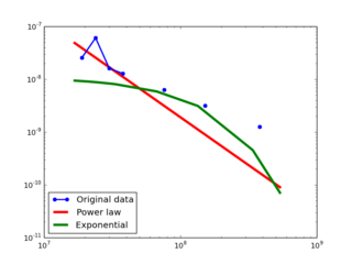
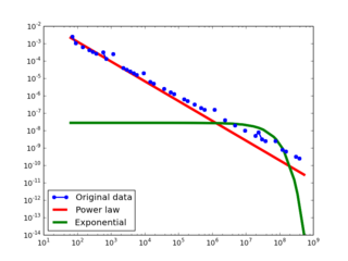
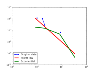
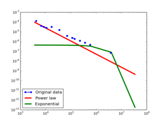
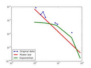
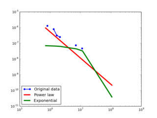
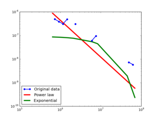
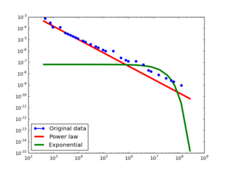
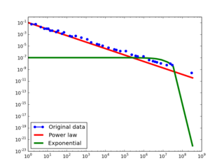
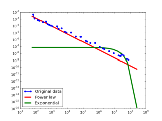
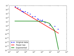
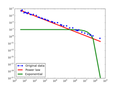
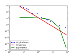
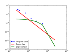
Here we plot the degree distributions of three approaches (LDM, NLAN, BI) on four RDF datasets.
For each dataset, we compute in-degree, out-degree, and total-degree distributions for LDM and NLAN approaches. BI approach has only total-degree distribution because it is undirected graph. We also compare the power law fit vs. exponential fit for each plot.
LDM
| DS | Degree type | alpha | xmin | sigma | R | p | D min | Tail coverage |
|---|---|---|---|---|---|---|---|---|
| BKR | in | 1.12 | 1 | 0.02 | 6.78 | 1.24E-11 | 0.15 | 60% |
| out | 1.23 | 1024 | 0.04 | 4.01 | 6.10E-05 | 0.14 | 28% | |
| total | 1.21 | 955 | 0.04 | 3.95 | 7.87E-05 | 0.13 | 58.33% | |
| YAGO2S | in | 1.11 | 1 | 0.02 | 6.33 | 2.52E-10 | 0.14 | 96.3% |
| out | 1.11 | 1 | 0.02 | 5.98 | 2.18E-09 | 0.14 | 96.3% | |
| total | 1.13 | 4 | 0.02 | 6.36 | 2.03E-10 | 0.12 | 92.31% | |
| DBPEDIA | in | 1.49 | 974383 | 0.13 | 1.76 | 0.08 | 0.11 | 25% |
| out | 1.46 | 524288 | 0.11 | 2.47 | 0.01 | 0.12 | 28.57% | |
| total | 1.13 | 16 | 0.02 | 5.38 | 7.39E-08 | 0.15 | 85.19% | |
| FREEBASE | in | 1.16 | 256 | 0.02 | 5.56 | 2.65E-08 | 0.11 | 70% |
| out | 1.81 | 16777216 | 0.26 | 1.54 | 0.12 | 0.12 | 16.67% | |
| total | 1.14 | 64 | 0.02 | 5.91 | 3.51E-09 | 0.12 | 79.31% |
BKR-SP
- LDM graphs transformed from the BKR-SP dataset
In-degree distribution.
Out-degree distribution.
Total-degree distribution.


YAGO2S-SP
- LDM graphs transformed from the YAGO2S-SP dataset

In-degree distribution.
Out-degree distribution.
Total-degree distribution.


DBPEDIA
- LDM graphs transformed from the DBPedia dataset
In-degree distribution.
Out-degree distribution.
Total-degree distribution.


FREEBASE
- LDM graphs transformed from the Freebase dataset

In-degree distribution.
Out-degree distribution.
Total-degree distribution.


NLAN
This table shows the parameters of the best power law distributions for each datasets using the NLAN approach.
| Dataset | Type | alpha | xmin | Dmin | sigma | R | p | Tail Coverage |
|---|---|---|---|---|---|---|---|---|
| BKR-SP | in | 1.933211288 | 895825 | 0.127628625 | 0.329940015 | 2.271051161 | 0.023143881 | 12.5% |
| out | 1.343236826 | 3705 | 0.115026299 | 0.083247158 | 3.894424558 | 9.84E-05 | 31.58% | |
| total | 1.21774704 | 491 | 0.141337886 | 0.041150323 | 3.228857504 | 0.001242858 | 58.33% | |
| YAGO2S-SP | in | 1.123959864 | 2 | 0.13926462 | 0.017708552 | 6.236336995 | 4.48E-10 | 92.31% |
| out | 1.145682633 | 8 | 0.12183686 | 0.029136527 | 4.997441147 | 5.81E-07 | 73.33% | |
| total | 1.128566546 | 4 | 0.132747188 | 0.019165569 | 5.732859944 | 9.88E-09 | 84.62% | |
| DBPEDIA | in | 1.648887842 | 970956 | 0.10993169 | 0.205196353 | 1.899457176 | 0.057504392 | 12.5% |
| out | 1.668078604 | 715028 | 0.128189532 | 0.222692868 | 2.574136552 | 0.01004906 | 0% | |
| total | 1.566221177 | 649090 | 0.147983393 | 0.163453975 | 1.774194648 | 0.076030959 | 12.5% | |
| FREEBASE | in | 1.176440054 | 410 | 0.117914742 | 0.028622356 | 4.937155187 | 7.93E-07 | 64.29% |
| out | 1.10925354 | 1 | 0.119199458 | 0.015007128 | 6.185548611 | 6.19E-10 | 96.3% | |
| total | 1.148300227 | 59 | 0.123663745 | 0.0223571 | 5.311427686 | 1.09E-07 | 77.78% |
BKR-SP
- NLAN graphs transformed from the BKR-SP dataset
In-degree distribution.
Out-degree distribution.
Total-degree distribution.


YAGO2S-SP
- NLAN graphs transformed from the YAGO2S-SP dataset
In-degree distribution.
Out-degree distribution.
Total-degree distribution.


DBPEDIA
- NLAN graphs transformed from the DBPedia dataset
In-degree distribution.
Out-degree distribution.
Total-degree distribution.


FREEBASE
- NLAN graphs transformed from the Freebase dataset
In-degree distribution.
Out-degree distribution.
Total-degree distribution.


BI
This table shows the parameters of the best power law distributions for each datasets using the BI approach.
| Dataset | alpha | xmin | Dmin | sigma | R | p | Tail Coverage |
|---|---|---|---|---|---|---|---|
| BKR | 1.201698959 | 491 | 0.127904446 | 0.037454556 | 4.762452101 | 1.91E-06 | 62.5% |
| Yago2s | 1.129751796 | 4 | 0.124153477 | 0.018728059 | 6.136824765 | 8.42E-10 | 92.31% |
| DBpedia | 1.381014259 | 524288 | 0.116475129 | 0.092409531 | 2.766134059 | 0.005672521 | 26.93% |
| Freebase | 1.684343461 | 24352099 | 0.105289281 | 0.216408404 | 2.006340037 | 0.044819981 | 13.79% |
Degree Distribution
- BI graphs transformed from four datasets
BKR total-degree distribution
YAGO2S-SP total-degree distribution
DBPEDIA total-degree distribution
FREEBASE total-degree distribution


Comparison
This table compares the power-law degree distribution of three type of graphs (NLAN, LDM, and BI) based on four RDF datasets (BKR, YAGO2S, DBPEDIA and FREEBASE. The values are the percentage of data points in each degree distribution that are covered by the power law. Distribution with higher percentage will better reflect power law distribution in the tail.
| DS | degree | NLAN | LDM | BI |
|---|---|---|---|---|
| BKR | in | 12.5% | 60% | NA |
| out | 31.58% | 28% | NA | |
| total | 58.33% | 58.33% | 62.5% | |
| YAGO2S | in | 92.31% | 96.3% | NA |
| out | 73.33% | 96.3% | NA | |
| total | 84.62% | 92.31% | 92.31% | |
| DBPEDIA | in | 12.5% | 25% | NA |
| out | 0% | 28.57% | NA | |
| total | 12.5% | 85.19% | 29.63% | |
| FREEBASE | in | 64.29% | 70% | NA |
| out | 96.3% | 16.67% | NA | |
| total | 77.78% | 79.31% | 13.79 |
LDM and NLAN
In general, LDM distributions have higher coverage percentage than the NLAN graphs. Out of 12 degree distributions, 9 LDM distributions have higher coverage than NLAN distributions while only 2 NLAN distributions have higher percentage. Both share the same coverage for BKR total degree distribution. Especially for all the in-degree and total-degree distributions, 100% LDM distributions have higher percentage than the NLAN distributions.
LDM and BI
2 out of 4 LDM graphs have significantly higher coverage percentage than the BI graphs, particularly in the total degree distributions of DBPedia (LDM: 85.19% vs. BI: 29.63%) and Freebase (LDM: 79.31% vs. BI: 13.79%).